Machine Learning | FIE Security Scanner

Dataset Construction

To construct our dataset, we compiled a collection of known malicious and benign Chrome extension IDs. Extension IDs were gathered in large batches using a third-party extension tool, Chrome-Stats.

Benign Criteria

Published on the Chrome Web Store by verified publishers
Store rating > 4.0 / 5
Low risk score according to Chrome-Stats' scoring metric

Malicious Criteria

Removed from the Chrome Web Store after being classified as malware

Total labeled samples

5,867

Malicious / Benign

3,001 / 2,866

Engineered features per sample

49

Train / Test split

80% / 20%

Each labeled extension was scanned using our feature extraction pipeline to produce a structured feature vector. We split the dataset into train/test before training to reduce leakage risk and ensure fair evaluation.

Feature Engineering

Our pipeline extracts static indicators from extension files and metadata. The goal is to capture behaviors commonly associated with malicious extensions — such as dynamic code execution, suspicious DOM manipulation, and risky external connections — using measurable, engineered features.

Examples of feature groups

JavaScript signals (dynamic code gen functions, suspicious objects, event handlers)
HTML/DOM signals (DOM operations, sinks density, iframe/form indicators, XSS vectors)
Statistical signals (string entropy, whitespace %, avg line length, keyword density)
Network/URL signals (external URL counts, http/https domains)

Implementation environment

Models were implemented in scikit-learn (Python). We used standard evaluation utilities and saved trained artifacts (e.g., via joblib). We also generated explanation plots (e.g., SHAP) to visualize global feature influence.

Random Forest: Feature Ranking and Model Selection

We used Random Forest as the main feature-ranking stage in our machine learning pipeline. Rather than using all extracted features directly, we first used Random Forest to estimate which features contributed most strongly to malicious-versus-benign classification, then passed the top-ranked subset into our final SVM-RBF model.

Step 1: Optimize forest size

To choose the number of trees, we trained forests from 15 to 500 estimators and measured out-of-bag error for each one. OOB error is computed from bootstrap samples and gives an internal estimate of how well the forest generalizes without requiring a separate validation split. We selected the forest size that minimized OOB error before running feature selection.

Selected forest size: 275 trees

Step 2: Select top-k features

With the tree count fixed, we ran 5-fold stratified cross-validation over feature subset sizes. For each fold, we trained a Random Forest on the training split, ranked the features by feature importance, selected the top k features, retrained the model using only those features, and evaluated performance on the validation split.

We repeated this process for every subset size from 1 to n and chose the value of k with the lowest average Mean Absolute Error (MAE) across folds. In our binary setting, this acts as an average prediction error measure over benign/malicious labels.

Selection metric: 5-fold CV MAE : 0.128

Step 3: Export ranked feature list

After identifying the optimal subset size, we retrained Random Forest on the training data, produced a final descending ranking of all features, and saved that ordering for later use. This ranked list became the basis for the feature subset used in our final calibrated SVM-RBF classifier.

SVM-RBF: Final Classification Model

We used a Support Vector Machine with an RBF kernel as our final classifier for malicious extension detection. The model was trained on a reduced input space of 39 Random-Forest-ranked features, allowing us to focus on the most informative static and behavioral indicators extracted from extension code.

The training pipeline consisted of StandardScaler followed by SVC(kernel="rbf"). Feature scaling was necessary because SVMs are sensitive to magnitude differences across input variables, and the RBF kernel was chosen to capture non-linear relationships that a linear separator would miss.

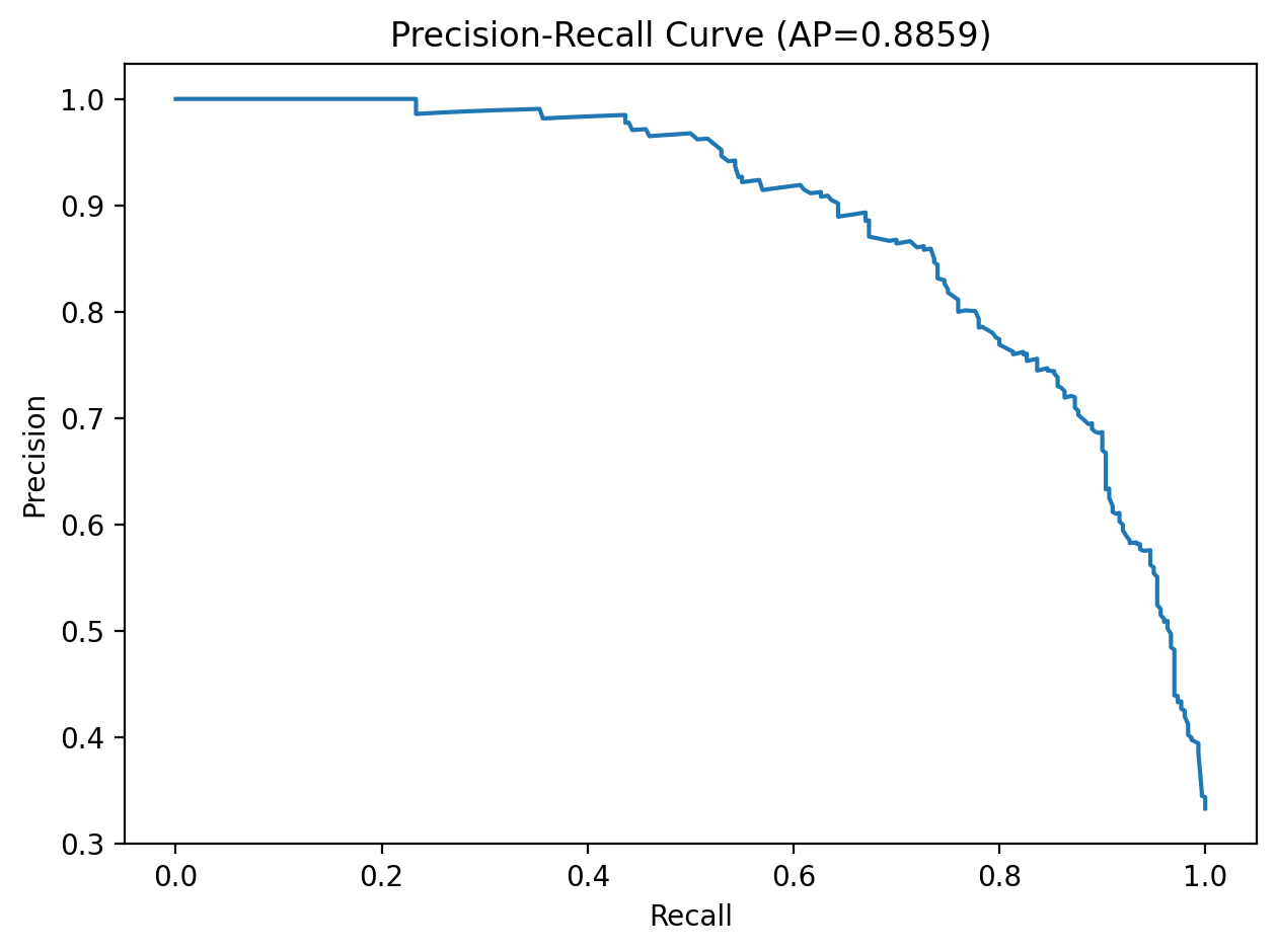
Model selection was performed with GridSearchCV over C, gamma, and class_weight using 5-fold stratified cross-validation. We optimized for average precision rather than raw accuracy so the chosen model would better handle class imbalance and prioritize malicious-class retrieval quality.

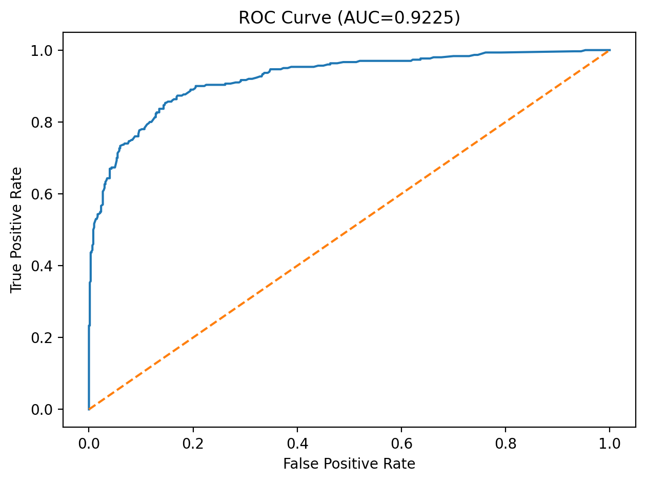
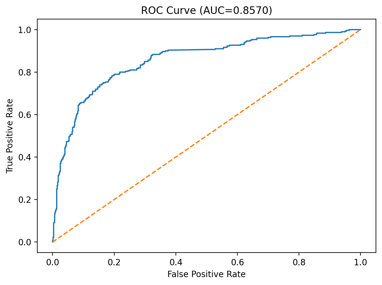
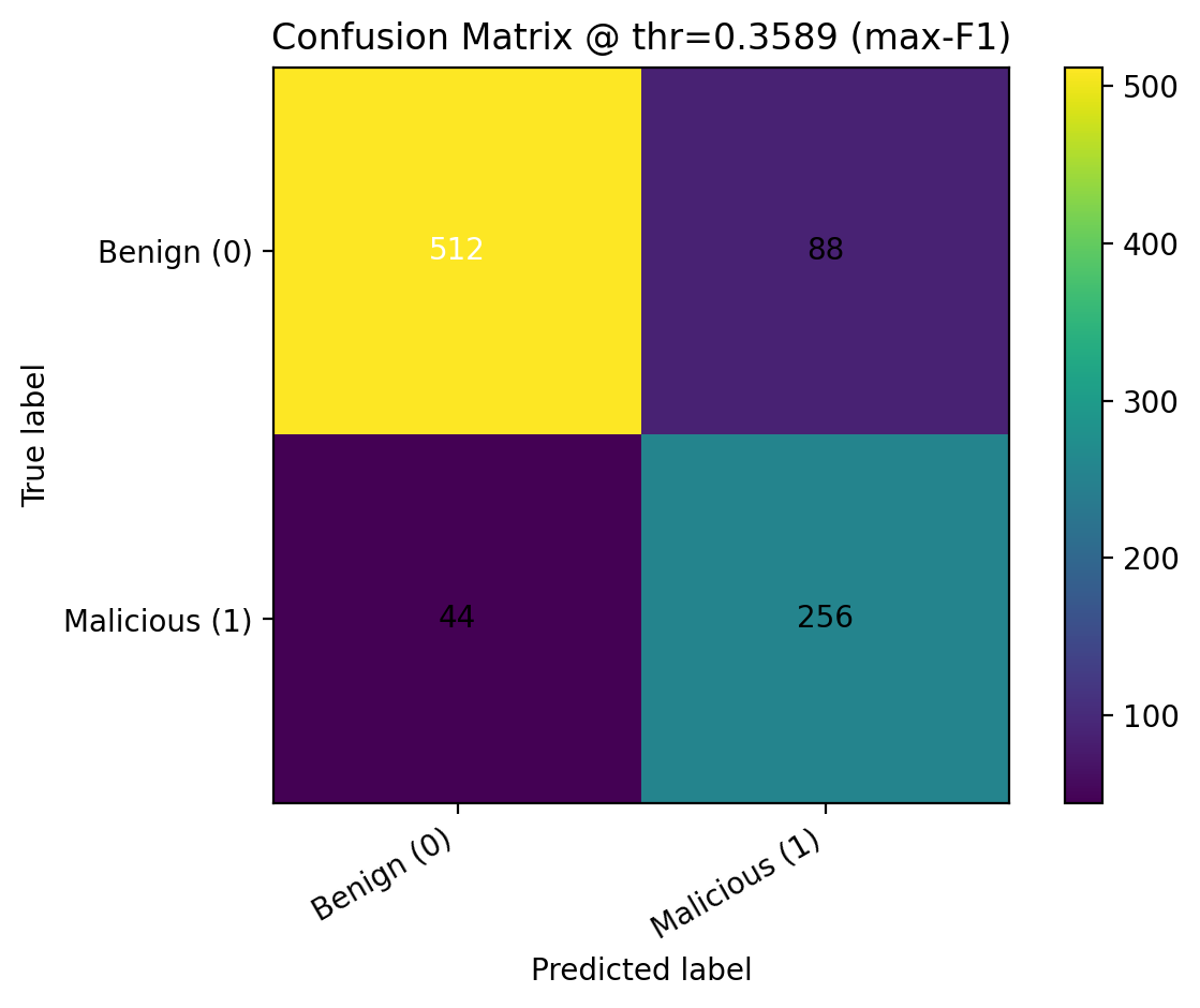
After training, we applied sigmoid probability calibration with CalibratedClassifierCV and evaluated threshold-free metrics such as ROC-AUC and PR-AUC, along with thresholded metrics including precision, recall, F1, balanced accuracy, and MCC. We compared predictions at the default threshold of 0.5, the max-F1 threshold, and a Youden’s J threshold, then saved the calibrated model, selected feature list, best hyperparameters, and final operating threshold into the deployment bundle.

Final feature subset: 39 features

Test Evaluation

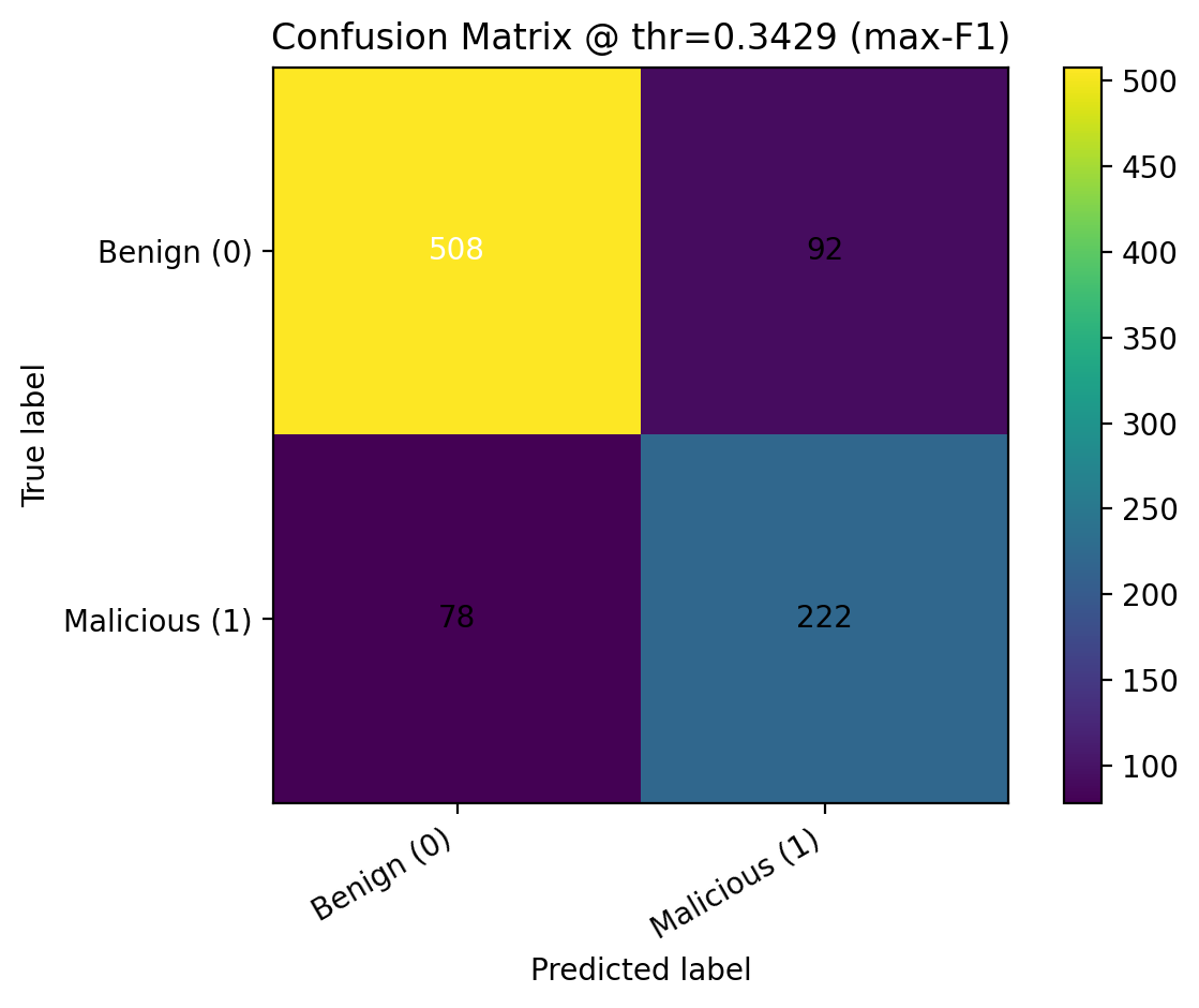
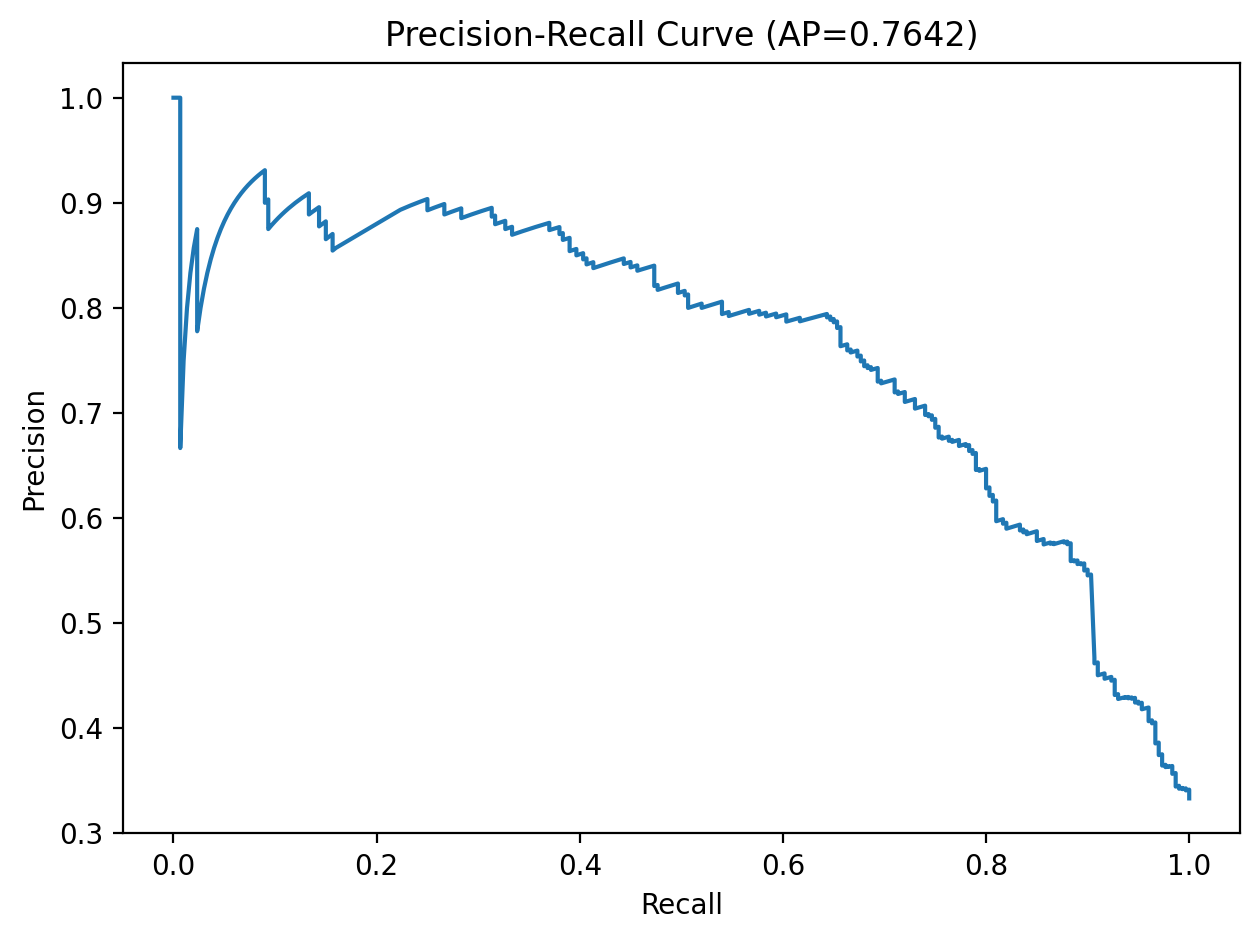
Below we report our final test-set performance. These values come from the evaluation artifacts generated in our training pipeline.

Key metrics (RF Test)

Accuracy: (0.853)
Precision: (0.744)
Recall: (0.853)
F1-score: (0.795)
ROC-AUC: (0.922)
PR-AUC / Avg Precision: (0.885)

Key metrics (SVM-RBF Test)

Accuracy: (0.811)
Precision: (0.707)
Recall: (0.74)
F1-score: (0.723)
ROC-AUC: (0.856)
PR-AUC / Avg Precision: (0.764)

Notes

In a malware detection setting, recall often matters because false negatives are costly. However, we also monitor precision to limit false positives. Threshold selection can shift this tradeoff.